Interaction of Two Spinning Dipoles

 

Introduction

 

A particular demonstration rig (see Figure 1), sometimes called "Whipmag", is comprised of a main rotor with several fixed, rotor-mounted permanent magnets and several smaller “satellite” rotors consisting of diametrally magnetized permanent magnets.  The satellite rotors spin when the central rotor spins due to magnetic coupling between the rotor and the stator magnets.

 

 

 

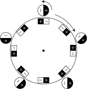
Figure 1: Schematic representation of Test Rig.

 

It has been surprising to some that the satellite rotors can stably rotate in either the opposite direction as the main rotor (i.e. rotating in a way analogous to the fashion that meshed gears usually rotate) or in the same direction as the main rotor wheel (in a direction that seems counterintuitive to those who conceptualize the arrangement as acting like a set of mechanical gears). Hobbyists have built replications that duplicate this behavior.  However, among the interested, there is no quantitative theory as to why the synchronization occurs.

 

The original device and its duplications are relatively complicated arrangements with magnets on the stator and many satellite wheels. However, the "gear-wise" and "anti-gear-wise" rotational synchronization can be understood by considering a related but much simpler topology – a pair of spinning dipoles. One spinning dipole is analogous to the main rotor in the more complicated experimental rig, and the second dipole is analogous to a satellite rotor. Dipole magnets are straightforward to analyze with closed-form mathematics, and the mechanisms that allow both "gear-wise" and "anti-gear-wise" rotation can be clearly demonstrated in this configuration.

 

Problem Geometry

 

The problem geometry is shown below in Figure 2.  The locations of the two dipoles are fixed in space, but the dipoles are free to rotate.  The geometry has the following attributes:

 

 

Figure 2: Problem geometry.

 

• The magnetization direction of both dipoles is always in-plane (i.e. has no component in the “z” direction pointed into/out of the page)
• Dipole 1 is fixed at point (0,0,0), and angle θ orients its magnetization direction.  Dipole 1 acts as the “drive” dipole—we could imagine that the dipole could be motored so that angle θ is increasing (the dipole is spinning) at a constant rate.
• Dipole 2 is fixed at point (l,0,0) and is oriented by angle φ.

 

The objective is to compute the torque on Dipole 2 due to Dipole 1 so that Dipole 2’s behavior due to the spinning of Dipole 1 can be understood.

 

Magnetic Field of a Dipole

 

The magnetic field of a dipole could be cribbed from a number of sources (e.g. http://www.intalek.com/Index/Projects/Research/MagneticForcesandTorq.pdf), but simply quoting the result is not very insightful. Instead, in this section, the magnetic field at Dipole 2 due to Dipole 1 will be derived from a point pole representation of Dipole 1.

 

Point poles act in a relatively intuitive way.  A point pole has a strength, q.  In a vacuum, flux flows away from the point pole in all directions.  The magnitude of the field intensity is proportional to the inverse-square of the distance from the dipole.  Mathematically, the field of a point pole located by vector r as viewed by an observer located by vector r_o is:

 

(1)

 

In (1), the first bracketed term represents the inverse-square decreasing amplitude of the field.  The second term indicates the direction of the field, flowing radially outward from the pole to the observer.  The magnetic permeability of free space is represented by μ_o.

 

A dipole can be modeled as being composed of two point poles of equal strength but opposite sign, as shown in Figure 3. The total field of the dipoles is the sum of the contributions of each pole. If the location of the first pole is r₁ and the location of the second pole is r₂, the relevant locations can be represented as:

 

(2)

 

where i and j represent unit vectors directed along the x- and y-axes, respectively.

 

 

Figure 3:  Dipole 1 modeled as two point poiles

 

Computing the field for each dipole from (1) for each pole and summing the results yields, for the field at the location of Dipole 2:

 

(3)

 

If it is assumed that δ is much smaller than l, the expression for flux density can be simplified by linearizing about δ=0 (i.e. turning the expression into one for a dipole, rather than for two discrete point poles.)  The resulting linearized expression for the magnetic field due to Dipole 1 at Dipole 2 is:

 

(4)

 

where m ≡ q δ is the magnitude of the magnetic moment of the dipole.

 

Interpretation of Magnetic Field Result

 

The magnetic moment of Dipole 1 as it spins about its axis is:

 

(5)

 

If the magnetic field from Dipole 1 at Dipole 2 were rotating perfectly gear-wise (and the angle of the field at Dipole 2 is the negative of the orientation of Dipole 1), we would expect the field to be proportional to:

 

(6)

 

However, the amplitude of the y-directed component of the magnetic field in (4) is only half the amplitude that would be expected for a perfectly gear-wise rotating field.  Instead, it can be verified by substitution that the field, B, can be represented as the sum of a gear-wise rotating field and an anti-gear-wise rotating field:

 

(7)

where

	(8)
	(9)

 

The torque, τ, on Dipole 2 is:

 

(10)

where

(11)

 

A dipole’s orientation tends to “latch on” to the orientation of a spinning field, since τ  goes to zero if B and m₂ are aligned.  Since the field seen by Dipole 2 is the sum of gear-wise and anti-gear-wise fields, Dipole 2 could latch on to either component and spin stably in either direction (so long as Dipole 2 has enough inertia and speed so that the displacement due to disturbance force due to the component turning in the other direction is not large enough to knock Dipole 2 out of synchronization).  Since the gear-wise field is three times larger in amplitude, this direction (φ = - θ) is the “preferred” direction of rotation.

 

Bearing Forces

 

To get some insight into the effects of rotation on bearing forces, it is of interest to compute the magnetic force on Dipole 2, in addition to the torque.  The definition for force on a dipole is: 

 

(12)

 

The force expression is written out on a component-by-component basis in matrix form as:

 

(13)

 

Multiplying the vector and matrix and putting the result back into vector form yields:

 

(14)

 

For "gearwise" rotations, φ = - &theta.  In this case, the steady-state part of the force (i.e. the part that is not a function of θ ) is:

 

 

(15)

 

For "anti-gearwise" rotations, φ =  θ.  In this case, the steady-state part of the force (i.e. the part that is not a function of q ) is:

 

(16)

 

For AGW rotations, the bearing force is much smaller.  Since bearing drag is related to bearing force, it is reasonable to expect that in an unpowered run-down, the GW rotation case would slow faster due to higher bearing drag.

 

Related Machines

 

The ability for a permanent magnet rotor to spin stably in either direction may seem like a rather unusual ability. However, this ability is an innate attribute of one of the simplest of electric machines, the single-phase permanent magnet motor.  The left side of Figure 4 schematically shows the layout of a common design of single-phase permanent magnet motor.  A diametrally magnetized magnet sits in the middle of a U-shaped core.  A single coil drives the iron and acts upon the magnet. 

Figure 4: Problem geometry.

 

It is fairly easy to see that this motor can spin equally well in either direction (practical implementations usually have geometric features in the poles to park the rotor so as to prefer a particular direction of rotation upon startup).  In terms of the previous development, the magnet could again be considered a dipole.  The rotor sees only a pulsating field in the x-direction: 

 

B = (Bcoil cos ωt ) i

(17)

 

where B_coil is the amplitude of the magnetic field at the magnet due to the current in the drive coil.  Just as before, this flux density, B, could be though of as the sum of clockwise and counter-clockwise components, either one of which the rotor could latch onto:

  

B = Bcw +  Bccw

(18)

 

where:

  

Bccw = (Bcoil cos ωt ) i + (Bcoil sin ωt ) j

(19)

 

Bcw = (Bcoil cos ωt ) i - (Bcoil sin ωt ) j

(20)

 

In some ways, this the behavior of this geometry is easier to "see" because the magnitude of the y-component of the B field is exactly equal to zero, rather than merely being relatively smaller.

 

There is no reason that the alternating field need be produced by a current-carrying coil.  The right side of Figure 4 shows the oscillating field being sourced by a second, spinning, permanent magnet, rather than an AC coil.  Again, the top magnet could spin stabily in either direction, either rotating or counter-rotating with the bottom magnet.

 

Conclusions

 

Although “anti-gear-wise” rotation might seem unexpected in a permanent magnet coupling, the mechanisms that allow this mode of rotation are in evidence even in very simple topologies.  That mechanism is a spinning field at the location of the “satellite” rotors in which the amplitude the field directed radial to the rotor has an amplitude that is different than the part of the field directed tangential to the rotor. The unequal amplitudes can be interpreted as the sum of fields that are rotating in different directions, implying that the satellite rotor could stably latch onto either direction of rotation.

 

Another interesting, experimentally observed, phenomenon is longer un-powered run-down times for rigs in "anti-gearwise" rotation.  By considering the bearing forces in the two-dipole configuration, it can be shown that the time-average translational force on Dipole 2 is lower in the "anti-gearwise" case, which should imply lower bearing drag and longer run-down times.